
Gradient optimization in HPLC is the systematic adjustment of a solvent program — its steepness, range, shape, gradient time, wash and re-equilibration — to obtain adequate resolution of the critical pairs in acceptable run time, with good peak shape and reproducible retention. It balances separation quality against throughput rather than simply making peaks elute faster.
A gradient method is also an instrument-dependent experiment. The composition entered in the method does not reach the column instantaneously: the system volume between where the gradient is formed and the column inlet creates a gradient delay. Optimization and method transfer must therefore consider both the programmed gradient and the gradient the column actually experiences.1
What is a gradient in HPLC?
In isocratic HPLC the mobile-phase composition stays constant during the separation. In gradient HPLC the solvent strength changes with time; in reversed-phase LC this usually means increasing the fraction of the stronger organic component, conventionally the mobile phase B. Weakly retained compounds can elute under the initial conditions, while progressively stronger solvent elutes more strongly retained compounds later in the run.
A complete gradient method contains more than the analytical ramp. It normally specifies initial conditions, an optional initial hold, one or more gradient segments, a strong-solvent wash where appropriate, a return to initial conditions, and enough re-equilibration before the next injection. Each of these is part of the method and each affects reproducibility.
AI Method Builder
Draft a starting method for your separation and refine it — save your work to your account.
What variables control a gradient separation?
A gradient separation is governed by a small set of variables that interact, so an optimization that fixes one can disturb another. Table 1 lists the main controls, what each one changes, and the usual first adjustment. The rest of this guide works through them in the order a method is normally developed.
| Variable | What it primarily changes | Typical first adjustment |
|---|---|---|
| Gradient range (initial and final %B) | Where analytes elute; early focusing and late washing | Move toward the useful elution window found in scouting |
| Gradient time, tG | Programmed steepness (Δ%B/tG); peak spacing and run time | Compare a shallow and a steep tG around the critical pair |
| Gradient shape | Distribution of solvent-strength change across the run | Start linear; segment only where a region needs it |
| Mobile-phase chemistry (modifier, pH, buffer, additives) | Selectivity (relative peak spacing) | Change when steepness alone will not resolve a pair |
| Temperature | Retention and, for some analytes, selectivity | Screen a few values alongside solvent chemistry |
| Flow rate, F | Effective steepness, efficiency and back pressure | Set with column dimensions; keep constant while tuning tG |
| Gradient delay volume, VD | When the gradient reaches the column; effective start conditions | Characterize per system; account for it on transfer |
What is gradient steepness (Δ%B/tG)?
For a simple linear program, the programmed gradient slope is the composition change per unit time:
Programmed gradient slope = Δ%B / tG
where Δ%B is the change in the strong-solvent fraction over the segment and tG is the gradient time (in %B per minute). For the same initial and final composition, increasing tG makes the programmed gradient shallower and decreasing it makes the gradient steeper. A shallower gradient often spreads analytes across a larger time window and can improve the separation of difficult neighbors, at the cost of run time; a steeper gradient compresses the chromatogram and improves throughput, but critical pairs can lose separation. Figure 1 illustrates the effect on a single conceptual mixture.
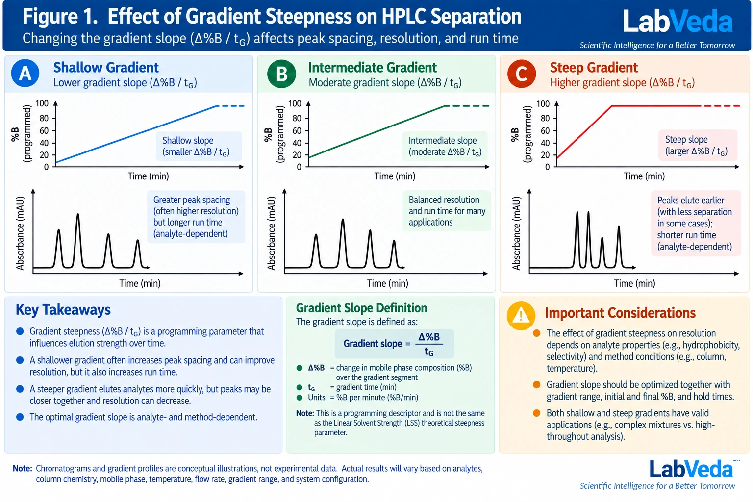
Δ%B/tG is a convenient programming descriptor, but it is not the dimensionless gradient-steepness parameter used in linear-solvent-strength (LSS) theory.2 The LSS steepness is commonly written in a form proportional to the analyte- and system-dependent quantities:
b ∝ S · Δφ · Vm / (tG · F)
where S is the analyte-dependent solvent-strength parameter, Δφ is the change in organic volume fraction, Vm is the column void (hold-up) volume, tG is gradient time and F is flow rate. Because the effective steepness depends on the column void volume, flow and S, two methods with the same %B/min can behave differently when column dimensions, flow, analytes or system characteristics differ.3 This is why scaling a gradient between column formats requires more than copying the slope.
How do you run a scouting gradient?
A broad scouting gradient is an efficient way to learn where a sample elutes before committing to conditions.4 A wide, relatively rapid gradient reveals the useful composition window; a second scouting run can then support a retention model built from scouting data that predicts how the separation responds to steepness.5 The generic 5–95% B program often quoted is a starting concept, not a universal prescription; the correct range depends on the sample, stationary phase and detector.
- Use a column and mobile-phase chemistry that are plausible for the analytes.
- Choose initial conditions that adequately focus and retain the earliest analytes.
- Run a sufficiently broad gradient to reveal the elution window of the relevant compounds.
- Identify the first and last analytes of interest and, above all, the critical pairs.
- Use the result to eliminate portions of the gradient that carry no useful separation information.
How do you narrow the useful gradient window?
If all analytes elute within a limited composition range, there is little value in spending most of the gradient outside it. Move the initial and final compositions toward the useful window while keeping enough margin for robust focusing, complete elution and column washing. Observing where peaks elute and then tightening the range and time is the standard way to remove wasted run time without sacrificing separation.4 Narrowing the range also changes the effective steepness over the region that matters, so the critical pairs should be re-checked after the range is moved.
How do you optimize gradient time around the critical pairs?
Once the useful composition window is known, gradient time is the logical next variable. Compare a small set of deliberately different gradient times while holding the other major conditions constant. The objective is not to maximize every pairwise resolution value; it is to reach adequate HPLC resolution for the critical pairs with acceptable run time and peak shape.
If a critical pair stays unresolved after reasonable changes in steepness, do not keep lengthening the gradient. The limitation is often selectivity rather than efficiency or time, and further gradient time buys little. Changes in stationary-phase chemistry, organic modifier, pH, buffer or temperature are then more productive than a shallower ramp.
How do you optimize selectivity, not just retention?
Retention changes are easy to see, but selectivity determines whether neighboring compounds actually separate. During development, watch whether the relative spacing of peaks changes when the composition range, solvent identity, pH, temperature or column chemistry changes. A method that merely moves an unresolved pair later in the chromatogram has not solved the separation problem.
The distinction is diagnostic. If all peaks shift together when a variable is changed, that variable is acting on global retention; if one pair changes its relative spacing, the variable is influencing selectivity (the separation factor) and is a candidate for optimizing the difficult pair. Selectivity-changing variables are the ones worth screening when steepness has reached its useful limit.
Should you use a linear, segmented, or curved gradient?
A linear gradient is usually the best starting point because it is easy to interpret and to transfer. Segmented gradients can then concentrate gradient time where difficult pairs elute and move quickly through regions that are already resolved. Curved gradients redistribute solvent-strength change across the run but can be more instrument- and software-dependent, so they must be documented precisely. Table 2 compares the common shapes.
| Shape | Description | When it helps |
|---|---|---|
| Linear | Constant programmed change in composition with time | Default; easiest to interpret, scale and transfer |
| Segmented linear | Different slopes in different time regions | Spend time on crowded regions, move fast through resolved ones |
| Convex / concave (curved) | Nonlinear composition change through the run | Occasionally useful; less transparent and more system-dependent |
| Step change | Abrupt jump in composition | Particular workflows only; justify against the separation |
What is a practical gradient-optimization workflow?
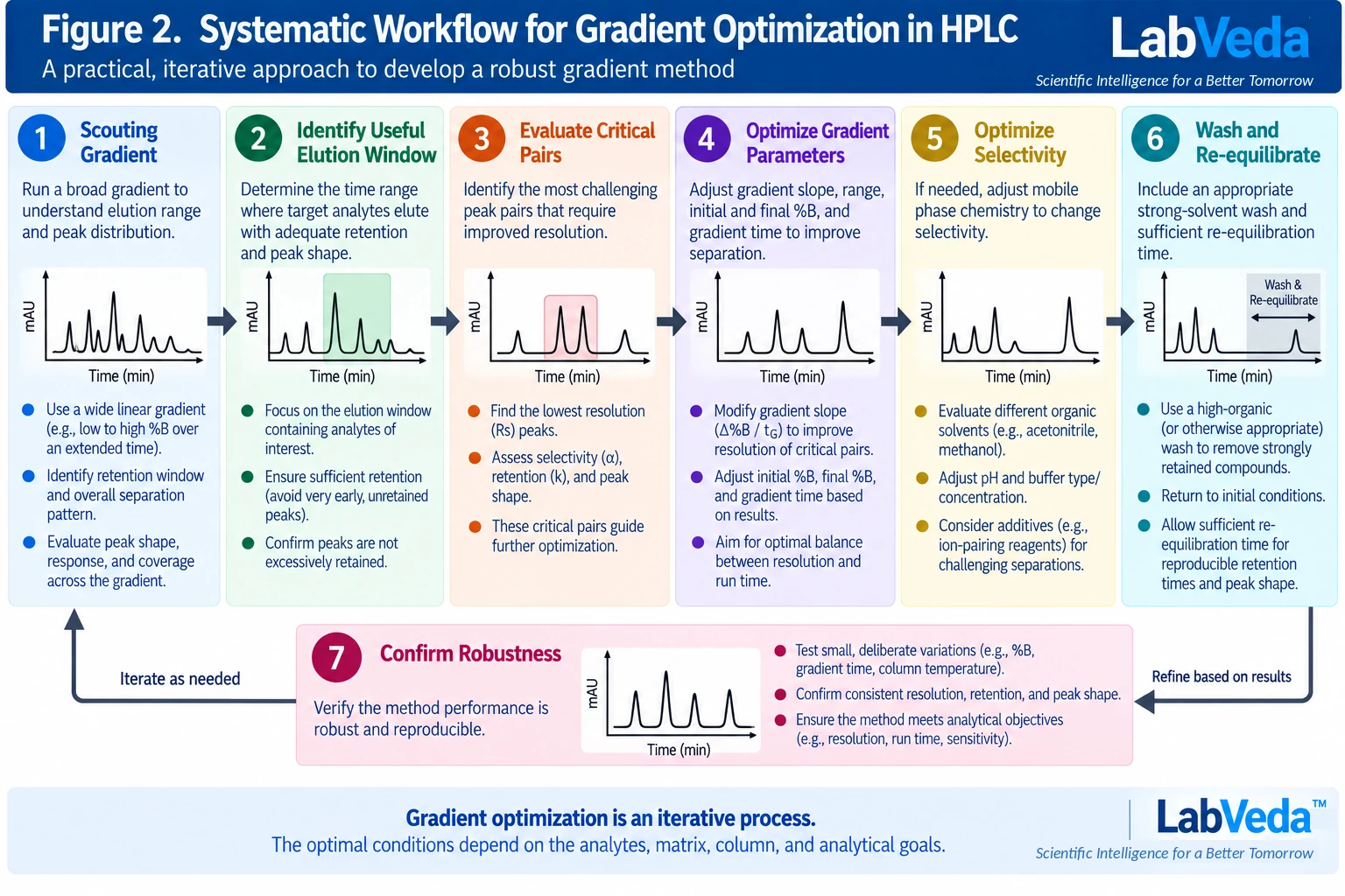
Gradient optimization is iterative, and a defined sequence keeps it from becoming trial and error. This gradient workflow is one part of the broader process of how to develop an HPLC method, which also fixes the column, mobile phase and detection. Figure 2 summarizes the workflow, and the steps below give the same sequence in order. Each step is revisited as later results come in; the aim at each stage is a decision, not a finished method.
- Define the analytical objective: critical analytes, required resolution, run-time target, detector constraints and robustness needs.
- Select plausible chemistry: column, organic modifier, aqueous phase, pH and buffer, and temperature.
- Run a scouting gradient: map the useful elution window.
- Focus the gradient range: remove composition regions that add time but little information.
- Vary gradient time: compare deliberately shallow and steep conditions around the critical pairs.
- Optimize selectivity: change chemistry, pH, modifier, temperature or gradient shape if critical pairs remain unresolved.
- Add wash and re-equilibration: ensure strongly retained material is removed and initial conditions are reproducible.
- Characterize system effects: know the gradient delay volume when transfer or fast gradients make it important.
- Challenge robustness: deliberately vary the relevant parameters within realistic ranges.
- Lock the method: document the full gradient table, system assumptions and acceptance criteria.
Why does gradient delay (dwell) volume matter?
Gradient delay volume (VD, often called dwell volume) is the system volume between the point where the gradient is formed and the column inlet. It delays the composition program the column experiences and can alter retention and selectivity on transfer between instruments.6 Figure 3 shows where it arises in the flow path. The corresponding gradient delay time is:
tD = VD / F
where VD is the gradient delay volume and F is the volumetric flow rate. A system with VD = 0.50 mL run at F = 0.50 mL/min imposes a delay of tD = 1.0 min before the programmed change reaches the column; the same method on a system with VD = 0.15 mL delays it by only 0.30 min, which is often enough to shift early-eluting pairs.
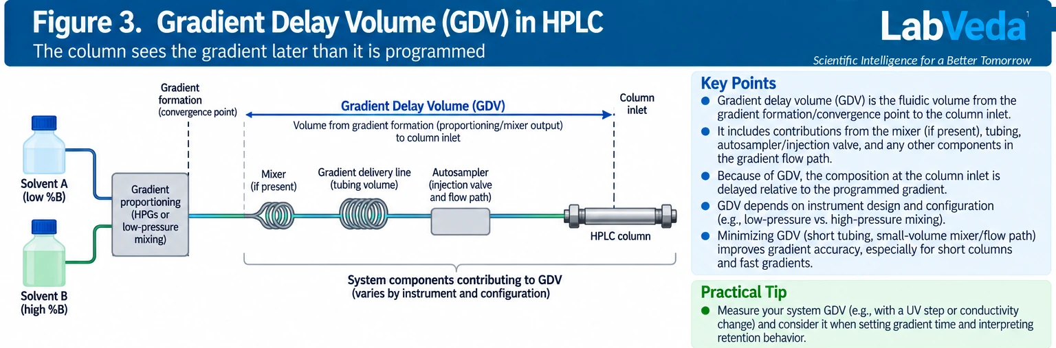
Because VD depends on instrument design and configuration, it should be characterized on both the source and target systems when a gradient method is sensitive to it, and considered when setting gradient time and interpreting retention.7 It can be measured with a UV step test in which a traceable marker is added to the strong solvent,8,9 and minimized with low-volume mixers and short, narrow tubing where fast gradients or short columns make the delay a large fraction of the run.
How do you separate gradient delay from extra-column dispersion?
When a gradient method changes after transfer, the first task is to determine what changed physically, because two distinct system effects are easily conflated. A difference in gradient delay shifts when the gradient reaches the column and can change the effective starting conditions and selectivity. Extra-column dispersion acts differently: tubing, connection and detector-cell volumes broaden the analyte bands and reduce the observed efficiency without changing the gradient composition profile. Figure 4 contrasts the two.
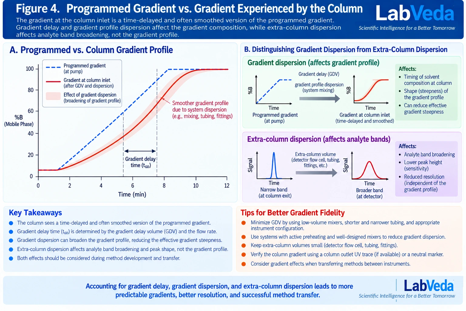
The practical consequence is a diagnostic order. If a transferred method loses resolution but the peak widths are unchanged, suspect a gradient-timing difference — delay volume or mixing — and adjust an initial isocratic hold or the gradient timing before touching the chemistry.7 If the peaks are broader and shorter across the board, suspect extra-column volume and check tubing, fittings and the detector cell. Treating a dispersion problem as a selectivity problem, or the reverse, wastes method-development effort.
Why is re-equilibration part of the gradient method?
After the strong-solvent portion of a gradient, the column and system must be returned to initial conditions well enough to give reproducible retention and selectivity for the next injection. The requirement depends on the stationary phase, the gradient excursion, the mobile phase, the column dimensions and the system volume. Full thermodynamic equilibrium is not necessary for every method; reproducible initial conditions are the practical criterion, and insufficient re-equilibration is a common cause of drifting retention times across a sequence.
A fixed universal number of minutes should not be copied between methods. Determine re-equilibration experimentally and express it in a way that stays meaningful when the method is scaled or transferred — column or system volumes rather than a wall-clock time — so the same reproducibility survives a change of instrument or column format.
What are common gradient-optimization failure modes?
Most gradient problems fall into a few recognizable patterns, each with a first variable to investigate. Table 3 maps the common symptom to its likely mechanism and the first corrective direction, following the diagnostic distinctions made above.
| Symptom | Likely mechanism | First corrective direction |
|---|---|---|
| Peaks span too wide a retention range under isocratic conditions | Sample too diverse for a single strength | Use gradient elution rather than isocratic |
| Useful peaks occupy only part of the scouting gradient | Range wider than the elution window | Focus the composition window; re-check critical pairs |
| Chromatogram globally compressed, pairs crowded | Programmed steepness too high | Increase tG (shallower gradient); re-evaluate |
| One critical pair unresolved despite steepness changes | Selectivity, not efficiency or time | Change modifier, pH, temperature or column chemistry |
| Method changes on transfer despite an identical gradient table | Different delay volume or mixing | Characterize VD; adjust an initial hold or timing |
| Retention drifts across repeated injections | Incomplete re-equilibration | Verify re-equilibration before changing the analytical gradient |
| Peaks broad and short across the whole run after transfer | Extra-column dispersion | Reduce tubing, fitting and detector-cell volume |
What should a transferable gradient method record?
A gradient method transfers reliably only if the record captures the conditions that materially affect the separation, including the system characteristics that shape the gradient the column sees.
- Column chemistry, dimensions and particle characteristics.
- Mobile phases, additives, pH specification and preparation procedure.
- Complete time/%B gradient table, including the initial hold, wash and return.
- Flow rate and temperature.
- Injection volume and sample diluent.
- Gradient delay (dwell) volume information when relevant.
- Re-equilibration conditions, expressed in column or system volumes.
- Critical-pair resolution or system-suitability criteria.
- Instrument-configuration details that materially affect gradient formation.
Frequently asked questions
Is a shallower HPLC gradient always better for resolution?
No. A shallower gradient often increases the time available for separation, but resolution also depends on selectivity, efficiency, the gradient range, analyte behavior, column chemistry and system effects. When selectivity is the limitation, extending gradient time provides little benefit and a selectivity-changing variable is needed instead.
How do I choose the starting %B?
Choose conditions that adequately retain and focus the earliest analytes without creating impractically long retention. The correct value is sample- and chemistry-dependent and is best found from a scouting run rather than copied from another method.
What is gradient dwell volume?
It is the system volume from the point where the gradient is formed to the column inlet, also called the gradient delay volume. It delays the composition change the column experiences by a time tD = VD/F, and can affect retention and selectivity, especially for fast gradients and short columns.
Why does my gradient method change when transferred to another HPLC?
Differences in dwell volume, mixing architecture, extra-column volume and temperature control can alter the effective gradient even when the programmed table is identical. Characterize the delay volume on both systems and check peak widths to tell a timing difference from an extra-column dispersion difference.
Should I optimize gradient time or column chemistry first?
Use a scouting gradient to understand retention, then decide whether the problem is mainly retention and time or mainly selectivity. Gradient time is the right lever when spacing can be improved by steepness; a persistent critical-pair problem usually needs a selectivity-changing variable.
How much re-equilibration is enough?
Enough to restore reproducible initial conditions for the next injection. Determine it experimentally for the column, mobile phase and system, and express it in column or system volumes rather than assuming one universal time.
The takeaway
Gradient optimization is a sequence of decisions, not a search for a single best slope. Scout to find where the sample elutes, focus the range on the useful window, then use gradient time to space the critical pairs — and when steepness stops helping, change selectivity rather than lengthening the run. Because the column experiences a delayed and slightly smoothed version of the programmed gradient, the delay volume and re-equilibration belong in the method and its record just as much as the gradient table does, and separating a gradient-timing problem from extra-column dispersion is what makes a method transfer predictably.
Developing a gradient method? A free LabVeda account saves your method-development sessions, diagnostics and exports across visits — the Knowledge Hub and tools stay open to everyone.
References
- L. R. Snyder, J. J. Kirkland and J. W. Dolan, Introduction to Modern Liquid Chromatography, 3rd ed., Wiley (2010).
- L. R. Snyder and J. W. Dolan, High-Performance Gradient Elution: The Practical Application of the Linear-Solvent-Strength Model, Wiley (2007).
- Agilent Technologies, “Essentials of Good HPLC Method Development” (27 July 2022). Covers LSS gradient steepness, gradient time, flow rate, column void volume and resolution.
- J. Lane / Agilent Technologies, “HPLC Method Development: From Beginner to Expert, Part 2” (28 March 2024). Covers reversed-phase gradient elution, gradient steepness and shape, method transfer and dwell-volume compensation.
- D. R. Stoll, “Initiating Method Development with Scouting Gradients—Where to Begin and How to Proceed?”, LCGC North America 41(5), 160–165 (2023). DOI: 10.56530/lcgc.na.jc4676g7.
- D. R. Stoll, “The Gradient Delay Volume, Part I: Theory”, LCGC International 1(1), 6–10 (2024). DOI: 10.56530/lcgc.int.wj6080e9.
- D. R. Stoll, “The Gradient Delay Volume, Part II: Practice—Effects on Method Transfer”, LCGC International 1(2), 6–10 (2024). DOI: 10.56530/lcgc.int.ia2675s7.
- Waters Corporation, “What is system dwell volume?”, Waters Knowledge Base WKB50711 (accessed 2026).
- Waters Corporation, “How do I determine system dwell volume?”, Waters Knowledge Base WKB50707 (accessed 2026).
Further reading
- D. R. Stoll, “The Gradient Delay Volume, Part III: Practice—Effects on Throughput”, LCGC International (2024) — extends refs. 6–7 to throughput.
- V. R. Meyer, Practical High-Performance Liquid Chromatography, 5th ed., Wiley (2010).
Reviewed against primary sources. Every definition, equation and working rule on this page is checked against the primary gradient-elution and method-transfer literature cited above. Numerical examples are illustrative calculations from the equations stated and are not method-development predictions or acceptance criteria. For validated or compendial methods, the applicable procedure and regulatory framework take precedence over the general rules of thumb given here. Evidence review: September 2026.