
If the concentration you calculate for the original sample changes with the dilution factor, the result is a pattern, not yet a cause. Before altering the method, verify the dilution arithmetic and confirm that every injected aliquot lies inside the calibrated range. Then compare matrix-matched dilution QCs, neat controls, analyte and internal-standard (IS) responses, and the effect of diluent, preparation timing and concentration. A result that rises after dilution can mean reduced matrix suppression or relief of high-response nonlinearity; a result that falls can mean adsorption, instability or low-end quantitation failure. Trend direction alone does not identify the mechanism.
How do you define the failure before changing the method?
For a sample diluted by factor D, the concentration estimated for the original sample is the measured concentration of the diluted aliquot multiplied by D:
Coriginal = Cdiluted × D
An illustrative original concentration of 100 units should therefore return measured concentrations of 50, 20 and 10 after 2×, 5× and 10× dilution, each of which recovers 100 when multiplied by its factor. Table 1 and Figure 1 show this expected behavior; the numbers illustrate arithmetic, not acceptance limits or experimental performance.
| Dilution factor D | Measured aliquot concentration (units) | Back-calculated original (× D) |
|---|---|---|
| 1× | 100 | 100 |
| 2× | 50 | 100 |
| 5× | 20 | 100 |
| 10× | 10 | 100 |
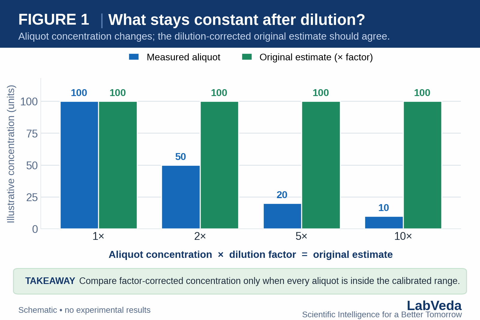
Compare back-calculated original concentrations, not raw peak areas alone. Record the matrix and diluent; whether dilution occurred before extraction, after extraction or immediately before injection; when IS was added; the analyte and IS peak areas; the calibration result before multiplying by D; the final result after multiplying; and the sequence position. A nominally identical factor can create a different chemical system if one workflow dilutes matrix before extraction and another dilutes an organic extract after extraction.
LC-MS PK Peak Integrity Engine
Interrogate carryover, matrix effects, ion suppression, and integration integrity before your PK data goes to QC.
How do you read the dilution pattern and design an experiment?
Figure 2 shows the three trend directions in dilution-factor-corrected concentration and the mechanisms each one implicates. An upward back-calculated trend means more diluted aliquots imply a higher original concentration. Reduced ion suppression as matrix load falls is one possibility. Another is upper-range response compression in a concentrated injection: a high-response sample may read low before dilution moves it into a better-behaved response region. Compare matched matrix and neat controls at appropriate concentrations and inspect raw response, calibration residuals, peak shape and the analyte/IS ratio before choosing between them. A stable isotope-labeled IS improves control of some variation but does not guarantee a linear response or eliminate nonuniform matrix behavior.1,2
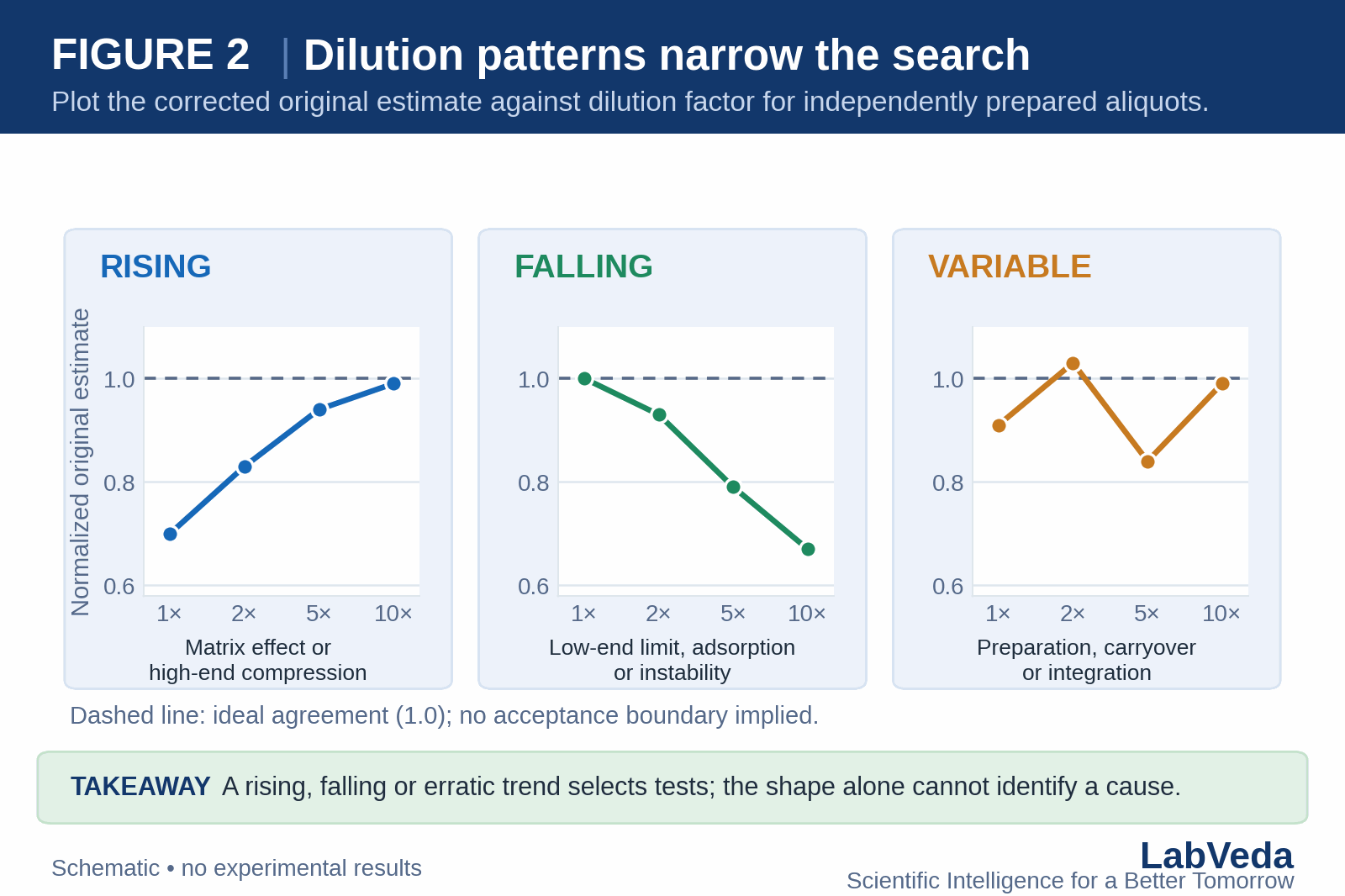
A downward trend can arise when losses become proportionally more important as analyte concentration falls, including adsorption to vials or wetted surfaces, instability, or measurement near the lower end of the range. A diluted aliquot that falls below the validated lower limit of quantitation (LLOQ) cannot be rescued by multiplying its unreliable concentration by a large dilution factor. Test fresh aliquots, controlled residence times, container material and matched controls. Adsorption is analyte and surface dependent; do not prescribe a universal solvent additive.3
Irregular results call for review of mixing, pipette volumes, dilution order, IS addition, extraction variability, integration and preceding injections. Carryover can especially distort a low-concentration aliquot after a high sample, a pattern also seen when peak areas change across a sequence. Repeat independently prepared dilutions and inspect blanks rather than assigning a mechanism from a single series.
How do you run a controlled dilution investigation?
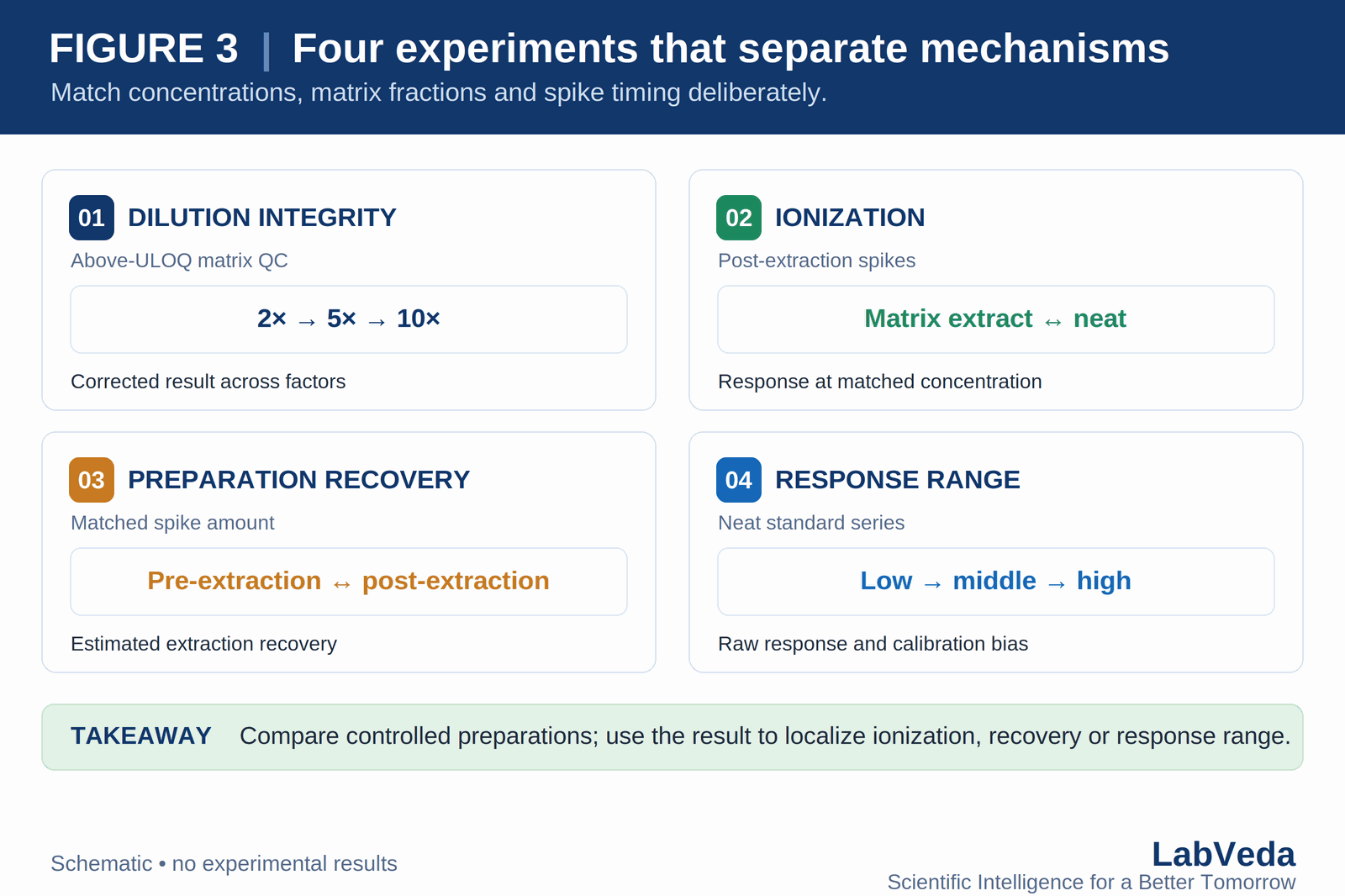
Start with a homogeneous high-concentration sample or independently prepared dilution QCs. Choose factors that bring the measured aliquots within the established calibration range. Prepare replicates at each factor, bracket the sequence with suitable QCs, and include a high-injection blank challenge if carryover is plausible. In a regulated chromatographic bioanalytical method, use the validated matrix-matched dilution procedure for reportable study samples; a solvent-dilution comparison can be a diagnostic experiment but cannot silently replace that procedure.4 Table 2 lays out four controlled comparisons and what each one can and cannot resolve, and Figure 3 summarizes their design.
| Question | Discriminating comparison | Observation that supports a hypothesis | What remains unresolved |
|---|---|---|---|
| Is the diluent or matrix load important? | Dilute above-ULOQ QC with appropriate blank matrix; compare exploratory neat or extracted-matrix controls at matched injected concentrations. | Dependence on matrix fraction supports a matrix-linked influence. | Ionization versus extraction or adsorption still needs localization. |
| Does ionization change with matrix load? | Compare post-extraction spikes in diluted blank extract with neat spikes at the same analyte and IS concentrations. | Different responses support matrix-dependent ionization. | It does not quantify pre-extraction recovery. |
| Does preparation change recovery? | Compare pre-extraction and post-extraction spikes under matched conditions and relevant matrix loads. | A preparation-dependent difference supports extraction loss or conversion. | It does not alone establish the identity of the surface or reaction. |
| Is the high end outside a suitable response range? | Measure a neat series and inspect raw analyte/IS response, peak height and area, calibration residuals and concentration-dependent bias. | Compression in neat standards supports an instrument/response-range contribution. | The matrix sample may also have matrix effects. |
| Is there a low-end loss? | Repeat fresh and aged aliquots in alternate suitable containers while staying in range. | A material- or time-dependent change supports adsorption or stability. | A separate validated stability assessment may be required. |
| Could a prior injection matter? | Run high → blank(s) → low, with appropriate control blanks and sequence positions. | A high-linked blank or elevated low supports carryover. | Localize injector, column or flow-path source. |
Why keep analyte and internal standard in the same investigation?
Plot raw analyte area, raw IS area, analyte/IS ratio and calculated concentration for every dilution. If IS is added before extraction, it can reflect preparation and ionization behavior differently from IS added to an already diluted extract. A matched stable isotope-labeled IS may correct a shared change, but differential suppression, cross-contribution, an unsuitable IS level or analyte-specific adsorption can leave the ratio biased. Inspect the actual calibration model and QC accuracy; a stable ratio by itself is not proof of dilution integrity.1,2
Do not infer that a curved calibration is automatically the remedy for poor dilution recovery. A regression change can hide a response-range, matrix or sample-preparation failure. Evaluate standards and QCs across the intended range and follow the method’s validation requirements before altering the response function.2,5
Where does ICH M10 apply to dilution?
ICH M10 addresses bioanalytical method validation and study sample analysis within its scope. For chromatographic methods, its dilution-integrity section evaluates whether diluting a sample above the upper limit of quantitation (ULOQ) with blank matrix preserves accuracy and precision. It calls for at least five replicates per dilution factor in one run, using factors and concentrations that cover those used for study samples, with mean accuracy within ±15% and precision no greater than 15% CV. The diluent should be the same matrix from the same species used for QCs; a justified surrogate may be acceptable for rare matrices. These are M10 criteria within that scope, not universal limits for every LC-MS/MS application.4
M10 separately describes dilution linearity for ligand-binding assays, including investigations of high-dose hook effects. Do not transfer that LBA-specific framework or language to a chromatographic LC-MS/MS method without evidence. For chromatographic analytical runs containing diluted study samples, M10 also addresses dilution QCs and how their acceptance affects the diluted samples.4
How do you correct the supported cause and verify it?
If matrix-dependent ionization is supported, investigate chromatographic separation, cleanup, an appropriate matrix-matched calibration strategy and IS suitability. Dilution may reduce matrix load but can also push analyte below the LLOQ; demonstrate the usable factor range rather than assuming that more dilution is better.1,6 Figure 4 maps each observed pattern to the discriminating test that comes next.
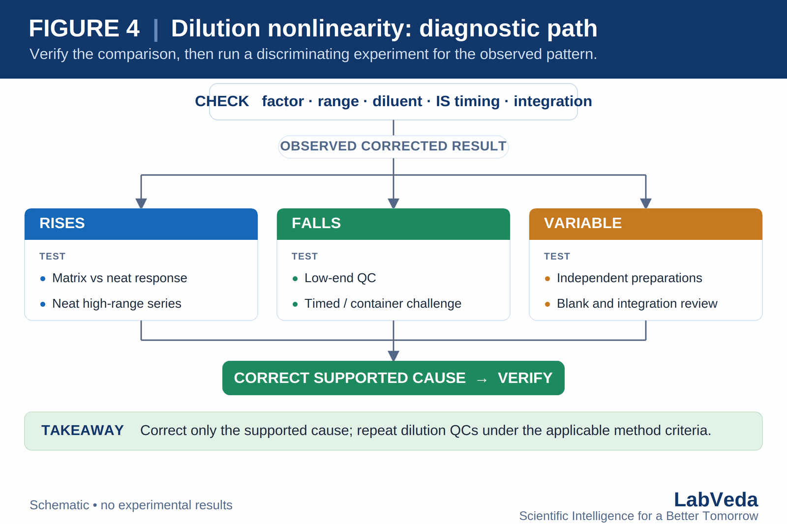
If a neat standard series shows response compression, adjust the validated calibration range, injected load or acquisition conditions as justified by method development.5 If pre-extraction recovery or adsorption is implicated, localize the affected preparation step or surface and verify a compatible change in materials or conditions.3 If carryover is shown, address the relevant wash path and confirm the high → blank → low challenge. If results are irregular, correct the preparation or integration failure and repeat independently prepared dilution series.
The endpoint is a reproducible result under the original challenge: relevant dilution factors, intended matrix lots and analyte range, matched QCs and blanks, and method-specific accuracy and precision. Do not accept a correction merely because one dilution happens to agree with the undiluted sample.4
Frequently asked questions
Why does my calculated concentration rise when I dilute an LC-MS/MS sample?
Reduced matrix suppression or relief of high-response nonlinearity are two possibilities. Compare matrix-matched and neat controls at matched concentrations, inspect raw analyte and IS behavior, and confirm every diluted aliquot is inside the calibration range before assigning a cause. The trend direction narrows the options but does not, by itself, identify the mechanism.
Does a straight calibration curve prove dilution integrity?
No. Calibration standards can fit a chosen response model while above-range samples fail the dilution step because of matrix, recovery, container or preparation effects. Test dilution QCs with the applicable method and factors rather than inferring dilution integrity from the calibration fit alone.
Can I dilute with solvent rather than blank matrix?
Solvent dilution can help diagnose matrix effects during development. For a chromatographic bioanalytical method within ICH M10, the validated dilution-integrity procedure generally uses blank matrix from the same species; reportable samples must follow the validated procedure or a justified, validated alternative.4
Is the LC-MS/MS dilution problem a hook effect?
A high-dose hook effect is a specific concern in some ligand-binding assays. A high LC-MS/MS response may instead be compressed by ionization, acquisition or detector behavior. Demonstrate the actual mechanism; do not use “hook effect” as a generic label for chromatographic nonlinearity.4,5
What if analyte and IS areas change together but the ratio is stable?
Check QC accuracy and the back-calculated concentrations. The shared change may be substantially compensated by the IS, but a stable ratio does not identify the cause or guarantee that other sample lots and factors behave the same way.1,2
The takeaway
A result that changes with dilution factor is a signal to investigate, not a mechanism to name. Verify the arithmetic and the calibrated range first, then let the trend direction — rising, falling or variable — select a discriminating experiment that separates matrix-dependent ionization, extraction recovery, response-range compression, adsorption or stability, and carryover. Keep the analyte and internal standard in the same investigation, honor the validated dilution-integrity procedure for reportable samples, correct only the cause the evidence supports, and confirm the fix against method-specific accuracy and precision across the relevant factors and matrix lots.
References
- G. Liu, Q. C. Ji, M. E. Arnold, “Identifying, Evaluating, and Controlling Bioanalytical Risks Resulting from Nonuniform Matrix Ion Suppression/Enhancement and Nonlinear LC–MS Assay Response,” Anal. Chem. 82(23), 9671–9677 (2010). doi:10.1021/ac1013018.
- R. Zhang, “Probing Liquid Chromatography–Tandem Mass Spectrometry Response Dynamics and Nonlinear Effects for Response Level Defined Calibration Strategies,” ACS Omega 9(1), 607–617 (2024). doi:10.1021/acsomega.3c06190.
- S. Warwood, A. Byron, M. J. Humphries, D. Knight, “The effect of peptide adsorption on signal linearity and a simple approach to improve reliability of quantification,” J. Proteomics 85, 160–164 (2013). doi:10.1016/j.jprot.2013.04.034.
- ICH, M10 Bioanalytical Method Validation and Study Sample Analysis, Step 4 guideline (2022). ICH guideline PDF; FDA final guidance: fda.gov.
- L. Yuan, D. Zhang, M. Jemal, A.-F. Aubry, “Systematic evaluation of the root cause of non-linearity in LC/MS/MS bioanalytical assays and strategy to predict and extend the linear standard curve range,” Rapid Commun. Mass Spectrom. 26(12), 1465–1474 (2012). doi:10.1002/rcm.6252.
- H. Stahnke, S. Kittlaus, G. Kempe, L. Alder, “Reduction of Matrix Effects in LC–ESI–MS by Dilution of the Sample Extracts: How Much Dilution is Needed?,” Anal. Chem. 84(3), 1474–1482 (2012). doi:10.1021/ac202661j.
Reviewed against primary sources. The mechanisms, experiments and interpretations on this page are checked against ICH M10 and the primary literature cited above. The figures are conceptual illustrations or calculated arithmetic, not experimental data, and no universal acceptable dilution or matrix-effect threshold is implied. For validated or compendial methods, the applicable procedure and regulatory framework take precedence over the general guidance given here. Evidence review: September 2026.