
HPLC method transfer is the controlled process of moving an analytical procedure from one instrument, laboratory or LC platform to another while demonstrating that the receiving system meets predefined transfer acceptance criteria. The central question is not whether the two instruments are physically identical; it is whether the target system reproduces the analytical performance the procedure requires, verified against criteria set before testing.
Because an instrument determines how nominal method conditions are physically delivered, two systems running the same gradient table, flow, temperature and injection can still expose the column to different fluidic, thermal and detection environments. Successful transfer is therefore a demonstration against criteria, achieved by diagnosing real instrument differences and making the smallest justified, permitted change — not by editing the method until the chromatogram looks familiar.
What is HPLC method transfer?
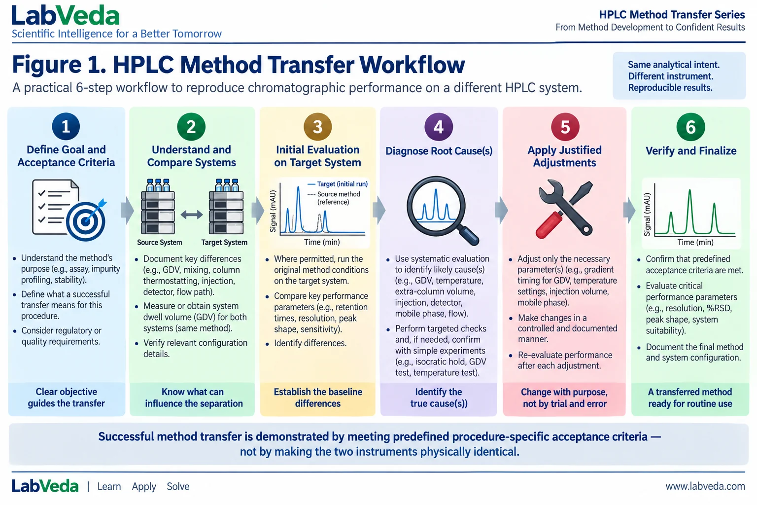
Method transfer moves an established procedure to a receiving environment — the same instrument model in another laboratory, a different vendor platform, or a migration from conventional HPLC to lower-volume UHPLC hardware — and shows that the target meets the procedure’s transfer criteria. Vendor method-transfer guidance from both Thermo Fisher and Waters emphasizes understanding the instrument differences that can influence chromatographic performance rather than assuming identical hardware.1,2,3,4 Figure 1 shows the six-step workflow this guide follows.
Chromatography Troubleshooting Decision Engine
Any HPLC symptom, one starting point — the engine narrows hundreds of failure modes to the few that fit your evidence.
Why can the same HPLC method behave differently on two instruments?
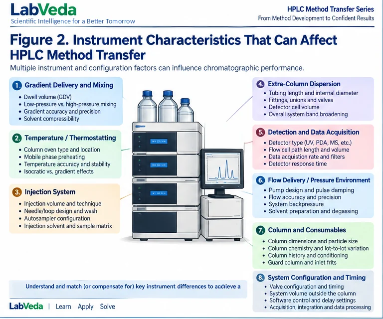
An LC method specifies nominal conditions, but the instrument determines how they are delivered. Method-relevant differences include gradient delay volume and mixing, column thermostatting and preheating, injection configuration, extra-column dispersion, flow-delivery and pressure environment, detector cell and acquisition settings, and the tubing, fittings and valves in the flow path.1,2 Which factor dominates depends on the procedure and the observed symptom. Table 1 lists the characteristics that most often change a transferred result, and Figure 2 maps them onto the instrument.
| Characteristic | What differs between systems | When it matters most |
|---|---|---|
| Gradient delay volume (GDV) and mixing | Fluidic volume from gradient formation to the column; mixer design | Gradient methods, fast gradients and short columns |
| Thermostatting and preheating | Oven type, mobile-phase preheating, frictional heating | Temperature-sensitive selectivity; platform migration |
| Injection system | Injection volume/technique, needle and loop design, wash | Peak shape and early-peak fidelity; solvent mismatch |
| Extra-column dispersion | Tubing length and i.d., fittings, detector cell volume | Small columns and low peak volumes (UHPLC) |
| Detection and acquisition | Detector type, flow-cell path length, data rate and filters, response time | Sensitivity, narrow peaks, quantitation |
| Flow delivery and pressure | Pump design, flow accuracy, pulse damping, pressure ceiling | Retention reproducibility; high-pressure UHPLC transfers |
| Column and system configuration | Column dimensions/lot, system volume outside the column, valve/timing | Any transfer; especially a change of column format |
How do you start — with intent and acceptance criteria?
Before comparing instruments, define what successful transfer means for the specific procedure: the analytes and critical pairs, the controlled method conditions, the system-suitability requirements, the relevant performance characteristics, and any regulatory or compendial constraints. Setting these first prevents the most common failure mode — changing the target method to make the chromatogram look familiar without showing that the change is necessary, permitted or aligned with the procedure.
How do you characterize the source and target systems?
For gradient methods, gradient delay volume deserves explicit attention. GDV is the fluidic volume between gradient formation and the column inlet, and it creates a time offset between the programmed gradient and the composition the column actually experiences,5 as covered in depth in the guide to gradient optimization and dwell volume. The corresponding delay time is:
tD = VD / F
where VD is the gradient delay volume and F is the flow rate; two systems with VD of 0.90 mL and 0.20 mL at 1.0 mL/min impose delays of 0.90 min and 0.20 min, a 0.70-min offset that shifts early-eluting peaks. Temperature also matters — thermostatting mode, preheating and frictional heating change the effective column temperature and therefore retention or selectivity — and extra-column dispersion becomes more important as column and peak volumes fall.1
Why evaluate the original method on the target system first?
Where the procedure, instrument compatibility and quality framework permit, run the target system on the original method conditions before making any compensatory change. This gives a diagnostic baseline and shows whether compensation is needed at all. If the result misses the predefined criteria, classify the difference before editing the method: a systematic shift of many gradient peaks points to a different set of causes than selective movement of a critical pair, generalized broadening, a pressure change or a response difference.
How do you transfer a gradient method and handle GDV?
A different configured GDV makes the same programmed gradient reach two columns at different times, so characterizing and, where appropriate, compensating for gradient-delay differences improves retention agreement on transfer.5 Compensation can use a programmed initial isocratic hold or a delay adjustment, sized to the measured GDV difference. But do not assume every retention difference is a GDV problem: flow accuracy, mobile-phase preparation, temperature, equilibration, column differences and composition errors produce similar symptoms, and a gradient-timing effect is not the same thing as extra-column band dispersion.
What about isocratic method transfer?
Isocratic methods have no programmed gradient delay, but instrument effects still matter. Flow accuracy, temperature, injection solvent and volume, detector settings, extra-column dispersion, mobile-phase preparation and column history can each change retention, peak shape, efficiency or response. The diagnostic discipline is the same: classify the symptom, compare the two systems, and correct the verified cause.
How do you change column dimensions or move from HPLC to UHPLC?
A transfer that changes column length, internal diameter, particle size or stationary-phase implementation is more than an instrument swap: flow, injection volume, gradient time, acquisition rate, pressure, temperature and extra-column volume may all need reconsidering, and several vendors treat these as coupled transfer parameters in a method-transfer calculator.6 To keep linear velocity comparable, flow scales with the square of the internal diameter:
F2 = F1 × (dc22 / dc12)
so moving from a 4.6 mm to a 2.1 mm i.d. column scales flow by 2.12/4.62 = 4.41/21.16 ≈ 0.21, i.e. a 1.0 mL/min method becomes about 0.21 mL/min at equal linear velocity. Gradient time is then scaled to keep the gradient volume proportional to the column volume:7
tG2 = tG1 × (V2 / V1) × (F1 / F2)
where V1, V2 are the column volumes. These scaling calculations give starting conditions only; experimental verification against the transfer criteria is still required.
How are compendial and validated methods different?
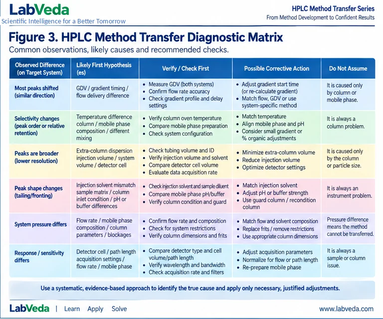
For USP compendial procedures, consult the current applicable General Chapter ⟨621⟩, the individual monograph and the laboratory’s quality and change-control framework before modifying chromatographic conditions.8 USP ⟨621⟩ contains provisions governing permitted adjustments in compendial use, but those provisions do not generalize to every validated method or transfer situation. For validated non-compendial procedures, whether a change is acceptable depends on the validation history, regulatory commitments and a change-control assessment — a chromatographically reasonable change is not automatically one that can be made without further qualification, verification or validation. Figure 3 and Table 2 give the symptom-based decision matrix that keeps a transfer diagnostic rather than trial-and-error.
| Observed difference | First hypotheses | Verify first | Possible action | Do not assume |
|---|---|---|---|---|
| Most gradient peaks shift similarly | GDV / gradient-timing / flow-delivery difference | Measure source and target GDV; flow; gradient program | Correct the identified timing/delivery difference if justified | Column failure |
| Only some peaks change relative position | Selectivity change | Temperature history; mobile-phase composition/pH; column | Correct the verified physical/chemical mismatch | GDV alone |
| Peaks broader or lower | Extra-column dispersion / acquisition | Tubing, fittings, detector cell/path length, data rate | Reduce unnecessary dispersion; correct acquisition | Gradient timing |
| Peak shape changes | Injection or sample-solvent mismatch | Injection volume/solvent; fittings; column inlet | Correct the verified injection/system cause | Stationary phase immediately |
| Pressure differs | Flow/temperature/viscosity/composition/system path | Flow accuracy; temperature; composition; tubing; column | Correct the verified cause within method constraints | Pump failure |
| Response / sensitivity differs | Detector / acquisition / injection | Wavelength, bandwidth, cell/path length, data rate, injection | Match the justified detection/injection conditions | Separation chemistry |
What is a practical transfer protocol?
- Freeze the source method and document representative reference performance.
- Define transfer acceptance criteria, critical pairs and system-suitability requirements before testing.
- Record the source-system configuration and method-relevant instrument characteristics.
- Configure and characterize the target system; characterize GDV for gradient methods when relevant.
- Where permitted and compatible, evaluate the original method conditions on the target system.
- Classify any difference: retention, selectivity, peak width/efficiency, peak shape, pressure or response.
- Investigate the physical or chemical cause using a symptom-based hierarchy.
- Apply the smallest scientifically justified and permitted correction.
- Repeat the experiment and verify the predefined transfer acceptance criteria.
- Document the system configuration, changes, rationale, results and any residual differences.
What are the common method-transfer mistakes?
Most failed transfers share a few habits: changing several variables at once before identifying the failure mode; assuming a retention shift means the column is different or damaged, when it is often drifting retention from timing or equilibration; using nominal system-volume specifications instead of measuring the configured GDV when the method is timing-sensitive; treating gradient-delay effects and extra-column band dispersion as the same phenomenon; ignoring thermostatting and preheating differences on platform migration; scaling column dimensions without reconsidering flow, injection, gradient time, acquisition rate, pressure and extra-column effects; and equating chromatographic similarity with regulatory acceptability without checking the applicable procedure and change-control requirements. Whether a spacing problem is efficiency or selectivity also decides which correction is even worth trying.
What does successful method transfer look like?
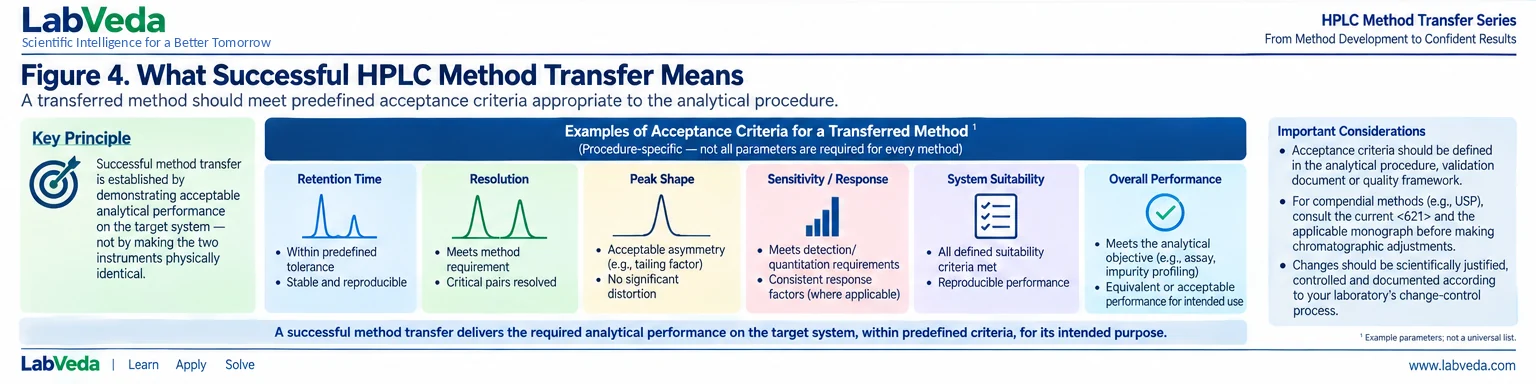
A transfer succeeds when the target system meets the predefined, procedure-specific acceptance criteria — which may cover retention within tolerance, adequate resolution of critical pairs, acceptable peak shape, precision, response and applicable system suitability — not when the two chromatograms merely look alike. Figure 4 shows the kinds of criteria a transferred method is judged against; the specific limits are always set by the procedure.
Frequently asked questions
Why does the same HPLC method give different retention times on another instrument?
Common causes include gradient delay volume, flow delivery, temperature, mobile-phase preparation, equilibration, column differences and timing. Diagnose the pattern — do many peaks shift together, or only some? — before changing the method.
Do I always need to compensate for dwell volume?
No. Characterize both systems and decide whether the difference materially affects the transfer criteria; some methods transfer acceptably without any GDV compensation, especially isocratic methods and slower gradients on longer columns.
Can I transfer an HPLC method directly to UHPLC?
Sometimes, but changing column dimensions or hardware brings in scaling, pressure, dispersion, acquisition, injection, temperature and GDV considerations. Treat it as a controlled migration with scaled conditions and experimental verification, not a straight copy.
What should stay the same in a transfer?
Preserve the controlled method conditions and the analytical intent unless a scientifically justified and permitted change is made. Exactly what may be adjusted depends on the procedure and its quality or regulatory context.
How do I know the transfer succeeded?
Demonstrate the predefined transfer acceptance criteria for the procedure, which may include applicable system suitability, critical-pair performance, precision and response — not merely a visual match of the chromatograms.
Is method transfer the same as method validation?
No. Transfer evaluates execution of an established procedure in a receiving environment; validation establishes the procedure’s performance characteristics. Whether verification or revalidation is needed depends on the specific change and the governing framework.
The takeaway
Method transfer is a demonstration, not a copy: the goal is to reproduce the analytical performance a procedure requires on a different system, measured against criteria set before any testing. Because the instrument, not the method file, decides how conditions are delivered, the reliable path is to define acceptance criteria, characterize both systems — GDV and temperature especially — run the original method on the target first, then classify any difference and correct the smallest justified, permitted cause before verifying against the criteria. Kept that way, transfer stays a controlled, evidence-based exercise rather than a round of trial-and-error method edits.
Transferring a method between instruments? A free LabVeda account saves your method-transfer diagnostics, sessions and exports across visits — the Knowledge Hub and tools stay open to everyone.
References
- Thermo Fisher Scientific, “An Instrument Parameter Guide for Successful (U)HPLC Method Transfer”, WP-72711.
- Thermo Fisher Scientific, “Successful and Stress-Free LC Method Transfers”, Method Transfer Application Compendium, EB-73812.
- Waters Corporation, “Using Gradient SmartStart Technology and an ACQUITY UPLC H-Class System to Emulate an Agilent 1100 Series LC System Separation for Impurity Testing” (application note, 2015).
- Waters Corporation, “Tools to Assist in Moving Established Methods to an Alliance iS HPLC System” (application note, 2024).
- D. R. Stoll, “The Gradient Delay Volume, Part II: Practice—Effects on Method Transfer”, LCGC International 1(2), 6–10 (2024). DOI: 10.56530/lcgc.int.ia2675s7.
- Thermo Fisher Scientific, LC Method Transfer Calculator (accessed 2026).
- L. R. Snyder, J. J. Kirkland and J. W. Dolan, Introduction to Modern Liquid Chromatography, 3rd ed., Wiley (2010).
- United States Pharmacopeia, General Chapter ⟨621⟩ Chromatography, USP–NF (current applicable text; consult the individual monograph).
Further reading
- D. R. Stoll, “The Gradient Delay Volume, Part I: Theory”, LCGC International 1(1), 6–10 (2024) — the companion to ref. 5.
Reviewed against primary sources. The transfer principles, the GDV and scaling relationships, and the compendial boundaries on this page are checked against the vendor method-transfer literature cited above, the LCGC gradient-delay-volume series, USP General Chapter ⟨621⟩, and standard LC references. Numerical examples are illustrative calculations from the equations stated and are not method-development predictions or acceptance criteria. For validated or compendial methods, the applicable procedure, monograph and change-control framework take precedence over the general guidance here. Evidence review: September 2026.